GPI and the BART

Recently, the BORG has been used to wrap the Berkeley Advanced Reconstruction Toolbox (BART) into a GPI node library for the purpose of allowing GPI users to easily explore and utilize this new compressed sensing library. This GPI-BART library is accompanied by some example networks that demonstrate basic wavelet based compressed sensing as well as some of the advanced joint compressed sensing and parallel imaging techniques that the BART package provides for MR reconstruction. This post gives an introductory overview of how the BART was wrapped in GPI and how the GPI-BART node library can be installed using the latest GPI v1.

The BORG

One of the new features in GPI v1 is the BORG interface which allows node developers to easily assimilate command-line tools for native use in GPI. The BORG, which stands for Building Outside Relationships with GPI, provides a simple wrapper interface that takes care of the file I/O required to communicate with external binaries. In the case of the BART, most of the tools require an input data file to process and subsequently produce a data file as an output. The BORG simply manages the temporary files required for this I/O. Reader and writer functions are required to translate the Python object (in GPI) to the appropriate file format for the command-line tool. In this case the BART comes with a Python library that translates their CFL/HDR file format to Numpy complex float arrays. This can be observed in the following code snippet of a GPI node that wraps the BART's traj command.

# load commandline tools
from bart.gpi.borg import IFilePath, OFilePath, Command
from bart.python.cfl import cfl # BART file format
...
    # grab user input from UI widgets
    x = self.getVal('readout samples')
    y = self.getVal('phase encoding lines')
    a = self.getVal('acceleration')
    r = self.getVal('radial')
    g = self.getVal('golden-ratio sampling')

    # assemble the argument string
    args = [base_path+'/traj']
    args += ['-x '+str(x)]
    args += ['-y '+str(y)]
    args += ['-a '+str(a)]
    args += r*['-r']
    args += g*['-G']
    args += d*['-D']

    # setup temp file for getting data back
    # from the external command
    out = OFilePath(cfl.readcfl, asuffix=['.cfl','.hdr'])
    args += [out]

    # run commandline and echo full command string
    print(Command(*args))

    # set GPI node output
    self.setData('trajectory', out.data())

    return 0

The example above starts with a local import of the BORG tools, which were developed in tandem with this node library. The GPI widgets values are then translated to command-line arguments, which are held as strings in a Python list object. Since the Traj node generates k-space trajectory coordinates, it requires an output file path to write out the trajectory data. The OFilePath object takes a reference to the file format reader function and generates a random temporary filename which is included in the arguments list. When the Command object executes with the argument list, it spawns a traj process and waits for it to finish and then it uses the reader function to convert the file to a Numpy array. The OFilePath object provides a reference to the Numpy via its data() method. Finally, when the OFilePath object falls out of scope it cleans up the temporary file on disk. The random filenames are important since the GPI canvas may contain multiple instances of the Traj node. The BORG interface simplifies this process which can save time when wrapping a large library like the BART.

For more examples, check out the wrapper nodes to the BART and FSL libraries.

Why a Fork?

The GPI-BART library is built off of a fork of the actual BART project. While the GPI wrappers could be considered a separate project, the BART project is currently undergoing a lot of development and the fork effectively ensures that the interface between the GPI wrappers and the BART is compatible. Another advantage is that this library can coexist with other BART installations on the same machine without interfering.

BART Data Conventions

The BART and GPI projects have a few key organizational differences in how they convey numeric arrays and k-space coordinates. In order to pass the data between nodes from each library, the data need to be manipulated to fit the each node's requirements. This is easily accomplished with the core GPI nodes. Lets start with an example of the worst case scenario: the traj node.

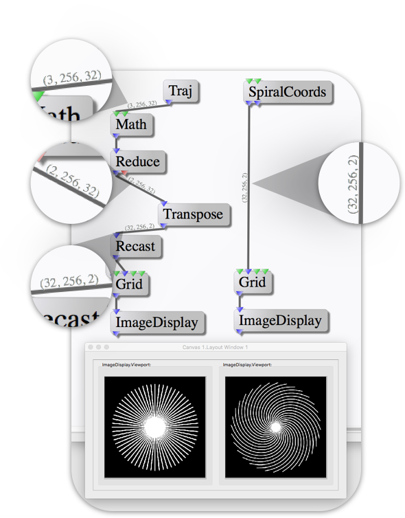
The image above shows an example gridded 2D radial trajectory (via the BART node library) and a gridded 2D spiral trajectory (via the GPI core library). Starting from the top nodes, you can see that the Traj node produces radial coordinates with dimensions [3, 256, 32] which is 3 cartesian coordinates, 256 sample points and 32 radial arms. The spiral coordinates from SpiralCoords are ordered [32, 256, 2] for 32 spiral arms, 256 sample points and 2 cartesian coordinates.

Step 1: Reduce Coordinates

Since this is a 2D trajectory, the Traj node passes zeros for the 'Z' coordinate and the SpiralCoords node passes 2 coordinates per point. In order to use the radial trajectory with the core Grid node, the 3rd coordinate of the array must be cropped out. This is accomplished with the Reduce node set to B/E where the '(B)eginning' index is 1 and the '(E)nding' index is 2. You can see that after Reduce, the Traj dimensions are [2, 256, 32].

Step 2: Transpose Dimensions

The Transpose node is used to flip the order that the trajectory data is organized in. After the Transpose node, the dimensions are [32, 256, 2], which matches the order of the spiral coordinates.

Step 3: Recast the Data Type

If you hover the mouse cursor over the coordinate port on the Grid node a tooltip will pop up with the data type required by that port. In this case, Grid can take floating point arrays with single or double precision. Hovering over the Traj output port shows that the array is of type complex float. In this case the trajectory definition only makes use of the real component so the imaginary component is set to zero. This can be directly recast into a float array without loss of data.

Step 4: Coordinate Scaling

You have noticed that the first node after Traj is Math. This is because the trajectory coordinate convention used in the BART is from N/2-1 to N/2 where N is the number of points along a dimension of the grid matrix. The GPI core library uses the convention of -0.5 to 0.5. So the coordinates are divided by the target matrix size via element-wise scalar division.

This example has shown how the BART and core GPI nodes can be easily adapted to communicate data between the two libraries using the stock data manipulation nodes in the core library. The conventions for data between these two libraries are different as would be expected between any two libraries that are developed independently. The goal for this example is to show that a cross library data transfer may require some extra attention.

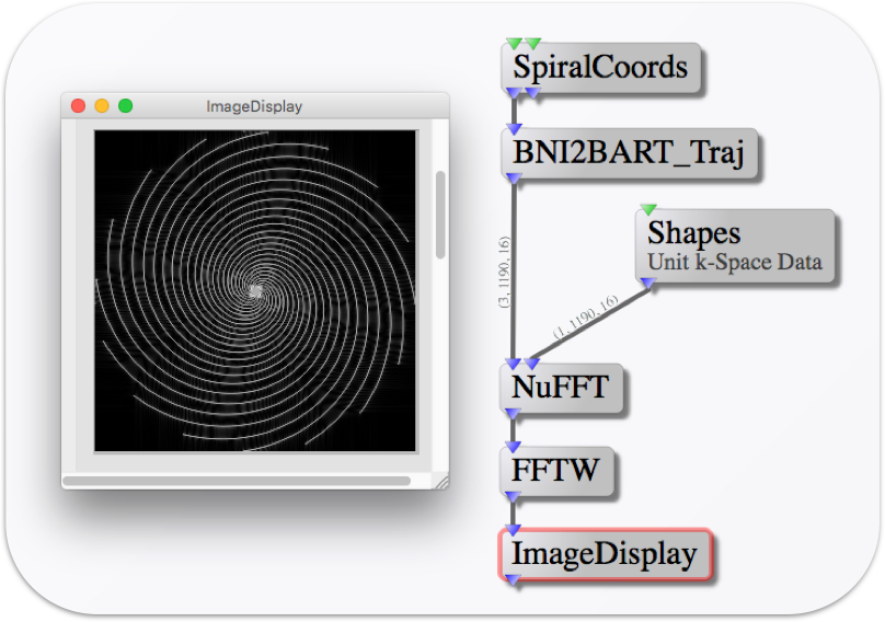
Another approach to this problem would be to integrate these differences into the nodes themselves. An example of this can be seen in the image above. The SpiralCoords node is generating a trajectory that is reformatted using the BNI2BART_Traj node (included in the wrapper library). This allows the coordinates to be directly used in the BART's NuFFT node.

GPI-BART Installation

There are two components to the GPI-BART node library installation: the BART compilation and the GPI node library installation. Before starting download or clone the GPI-BART fork:

First (if you haven't already), make a 'gpi' directory in your home directory. If you're not sure why you'd do this, checkout the post Installing Node Libraries.

    $ cd ~/
    $ mkdir ~/gpi
    $ cd ~/gpi

Next, use git to clone the node library project into a directory called 'bart'.

    $ git clone https://github.com/nckz/bart.git bart

BART Compilation

The BART compilation instructions can be found in the README.md in the base directory of the project source code. To summarize, the BART has some third party library dependencies that are specific to each OS (e.g. Mac OSX). For OSX, the Xcode and the gcc compiler must be installed before the make command can be issued. Once you've installed the dependencies, make the BART.

    $ cd ~/gpi/bart
    $ make

This will make the BART command-line executables, which will be accessible from the ~/gpi/bart directory.

Installing Node Libraries

The BART compilation instructions above basically install the BART under a GPI node library directory structure. GPI will look at the ~/gpi/bart directory as if it where a Python library. In our fork, we've included the GPI wrapper nodes under the bart/gpi directory. This fixed directory structure allows the wrapper code to maintain the relative paths for the BART executables. Since the GPI wrappers are pure Python, they don't require compilation. If your GPI installation is setup with the default paths then GPI-BART library is ready to go.

If you have path modifications in your ~/.gpirc file or the nodes are not visible in your library menu, consult the Configuration docs or check out the post on Installing Node Libraries.

Events

This work has been presented at the ISMRM Workshop on Data Sampling & Image Reconstruction in Sedona Arizona this last January and will be presented at the ISMRM Annual Meeting & Exhibition in Singapore this March.

Thanks

We'd like to thanks the BART developers at UC Berkeley for their help in building these nodes.