As part of our GPI demo at at the ISMRM 2019 Open-Source Software Tools for MR Pulse Design, Simulation & Reconstruction Weekend Course, we've revived an example of BART working inside GPI. This example is intended to demonstrate the flexibility and capabilities of GPI to integrate other packages. This demo also highlights the use of GPI as a teaching tool; the example is based on this example from Professor Lustig.

Before getting started here, please see Nick's post on setting up GPI for the ISMRM 2019 demo.

Download and Compile BART for GPI

BART for GPI is a fork of the BART project. We concede this fork is out of date, but it should suffice for a demonstation. Updating to a newer version would be fairly trivial for someone familiar with both BART and GPI. Check out Nick's other post on how BART was wrapped for use in GPI if you're interested in making this work.

First, prepare your virtual machine for BART compilation:

> sudo apt-get install git gcc make libfftw3-dev liblapack-dev libpng-dev

If you're using the GPI ISMRM 2019 demo VM or AMI on EC2, the password for the ubuntu user is gpilab.

Next clone the BART for GPI fork into your gpi library folder:

> git clone https://github.com/nckz/bart.git /home/${USER}/gpi/bart

Finally, build and test BART:

> cd ~/gpi/bart
> make
> ./bart bench

If you're not working in the GPI VM, instead follow the instructions in the BART for GPI README.

Launch GPI and Open the Example

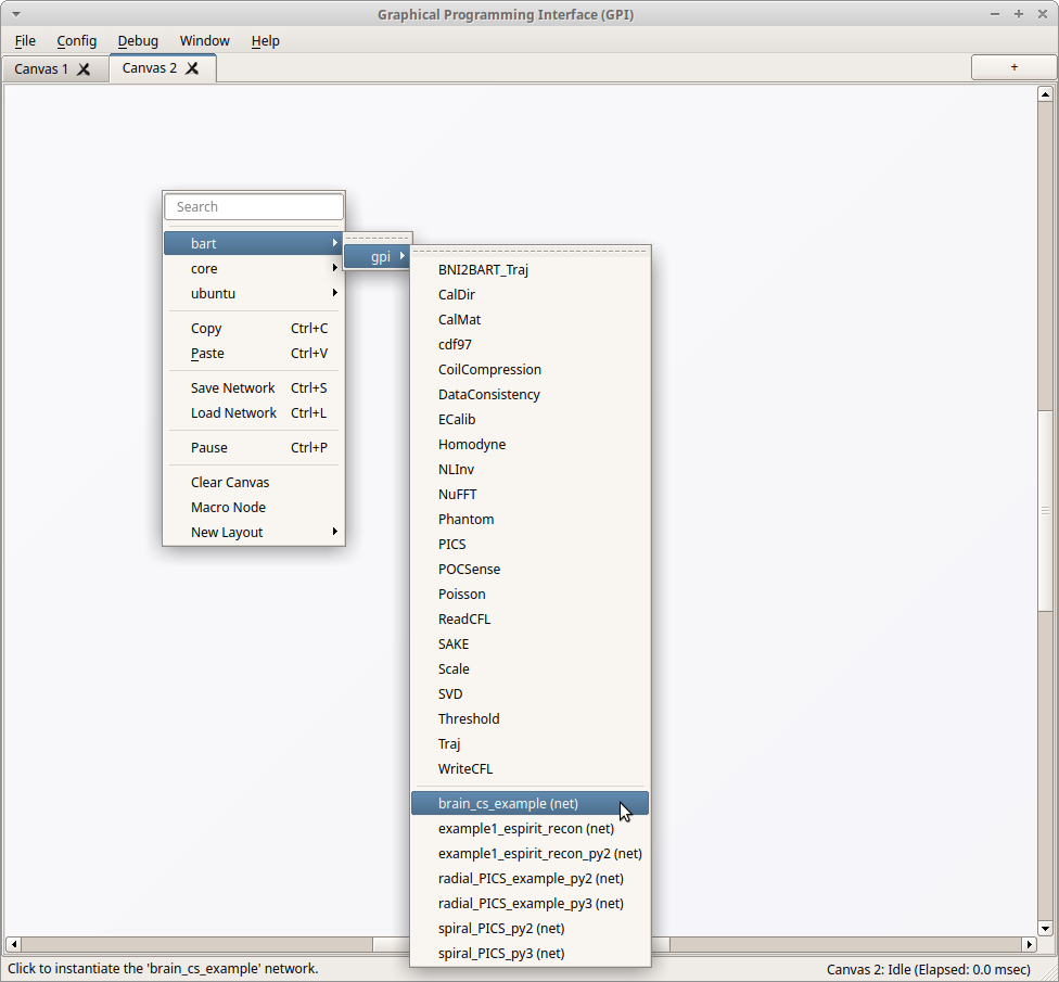
Open GPI using the startup script or from a terminal. Right click anywhere on the canvas and you should see a new Library in the menu called bart. GPI Libraries can contain both nodes and networks. Most BART functions should have corresponding nodes here, but for now go ahead and select the brain_cs_example (net) near the bottom of the menu.

The demo network will be loaded on the canvas, and the DownloadFile node should begin downloading the example data. This data (about 5 MB) will be stored in a temporary file.

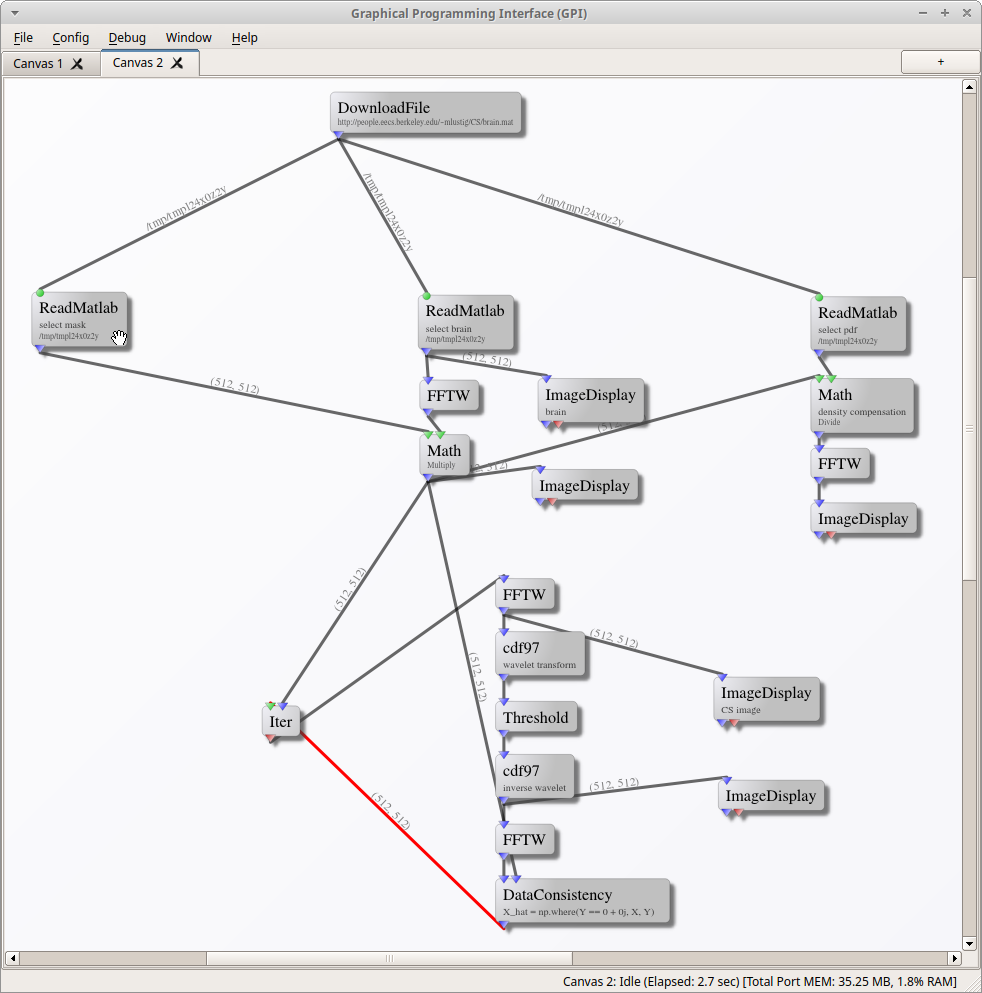
Configure and Run the Network

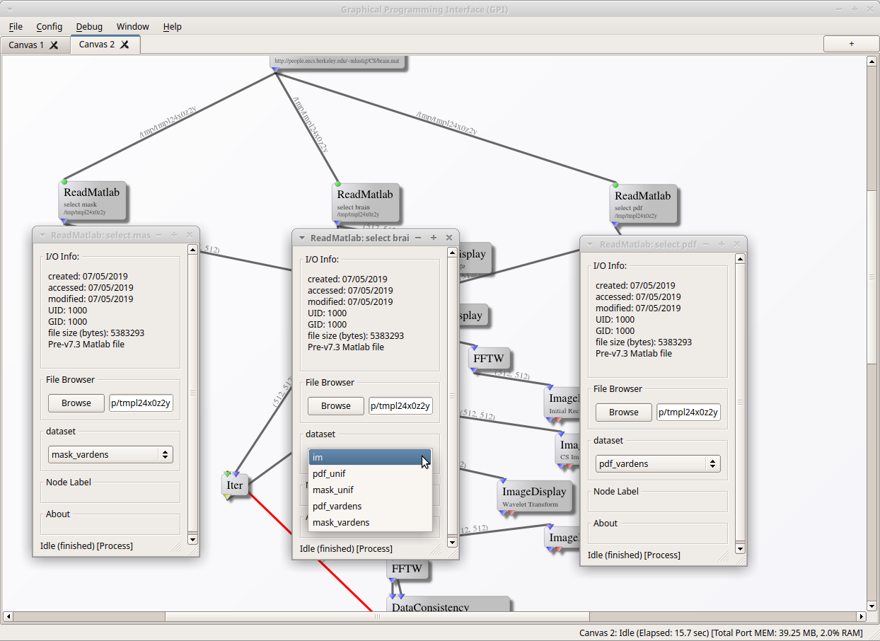
Note the three ReadMatlab nodes. Each is reading data from the same file (the one downloaded by the DownloadFile node) which contains several arrays. Right-click on each of these nodes to open their node menus. In the menu you will be able to select which array is output. From left to right we need to select the sampling mask, the image, and the sampling pdf.

Right-click on a few of the ImageDisplay nodes to probe the algorithm at various points. The ImageDisplay node labeled CS Image is the compressed-sensing reconstruction (though at this point it is only the inital condition based on zero-filling).

Open the Iter node and click the "Start/Stop" button to begin the iterative reconstruction. The CS Image will be updated with each iteration, and you can watch as the undersampling artifacts are removed by the wavelet-based soft-thresholding constraint.

There you have it! Explore the rest of the BART tools in GPI and let us know if you come up with any cool examples.